Taming the LIDAR Beast with MapD
Download HEAVY.AI Free, a full-featured version available for use at no cost.
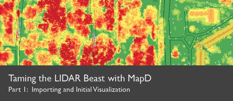
GET FREE LICENSEIn this post, I’ll describe how to import LIDAR data into MapD and do some simple visualizations of massive point datasets. In a subsequent post, I’ll show how to “enrich” traditional GIS data with valuable 3D attributes using MapD’s new geoprocessing capabilities.
Note: A Jupyter Notebook containing full code examples will shortly be available.
What is LIDAR?
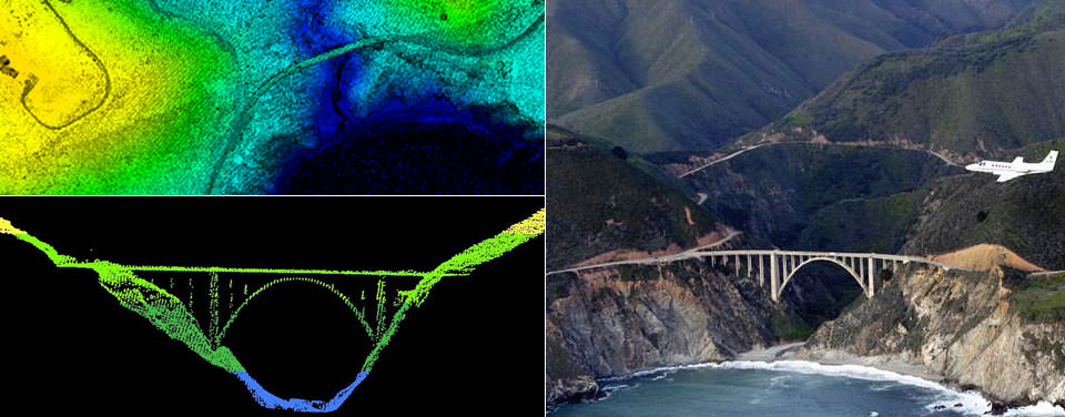
LIDAR (light detection and ranging) is rapidly-emerging form of “reality capture.” Available from either ground, vehicle or aerial sensors, LIDAR provides 3D point clouds describing the surfaces of objects and the planet, in considerable detail. As an active sensing product, it has the ability to “see through” clouds, and measure the heights of millions of objects. However this data is often not used to its full potential.
This is mostly because LIDAR data is typically huge, and its technical structure as captured and delivered is not immediately useful in common geospatial, database or business intelligence applications.
The Challenges
In dealing with LIDAR data, you will likely encounter a few common challenges:
- Finding such data in the first place
- Folders full of illegibly-named files in obscure formats
- The need to convert coordinate systems and merge tiles
- Difficulty manipulating & interpreting the data due to its sheer size
Fortunately, a scalable SQL database with GPU computing provides some good solutions. So let’s take those challenges one by one. Once you have your data in MapD, you’ll be able to deal with LIDAR as a single well-structured table, with interactive performance on huge datasets.
1) Finding LIDAR Data
There are many sources of LIDAR data, including many local governments. In general, LIDAR data are provided in two formats sanctioned by the International Society of Photogrammetry and Remote sensing (ISPRS): LAS and LAZ. By searching for files with those extensions, you can find and identify LIDAR data.
The current best US domestic and international indices of LIDAR data include:
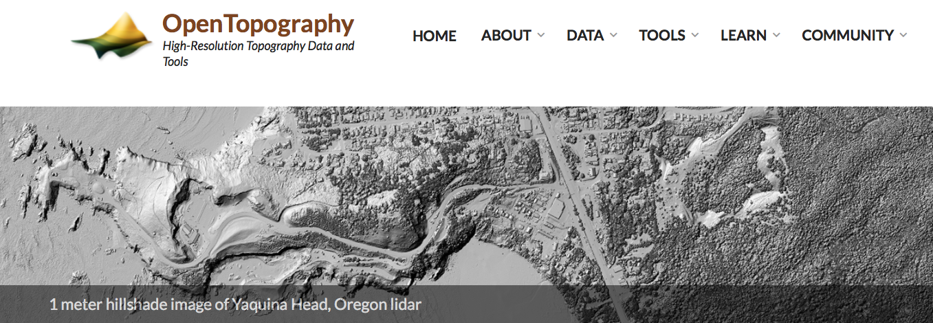
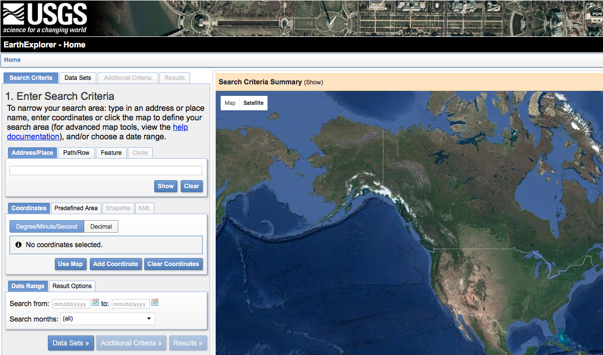
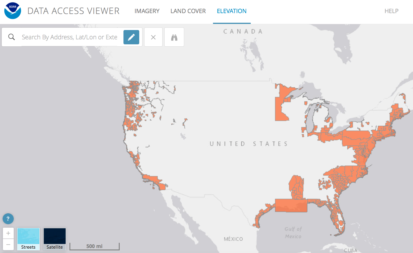

Wikipedia Page Indexing National LIDAR Datasets
2) LIDAR File Formats and Local Coordinate Systems
As noted, LIDAR data is typically provided in one of two specialized formats: LAS and LAZ. LAS is a text-based format for which more support libraries are currently available. LAZ is an emerging standard, hugely more efficient, but not yet as widely supported. Importantly, LAZ is not simply a zipped version of LAS, but actually has a format-specific compression system.
The immediate stumbling block is that neither file format is directly supported by MapD, or by the GDAL utility library which is available on all MapD installs.
There are multiple available tools which support conversion of LIDAR files to formats readable by MapD. However, we found that the easiest option is PDAL. PDAL is a fully open sourced library which provides a Docker image for easy installation. Full docs can be found here: https://pdal.io
PDAL also solves the second common issue mentioned above, which is local coordinate systems. MapD 4.0 supports the two most common global coordinate systems - web mercator and geographic latitude/longitude, both with WGS84 datum. In most cases, you’ll want to project LIDAR data from local coordinates to one of these two systems. In some cases, you’ll also need datum shifts, such as from NAD83 data. Note that you may lose some precision in doing so, due to the intrinsic limits of global coordinates, and some storage efficiency measures inside MapD.
So without further ado, here’s a single command which performs most everything you are likely to need:
!sudo docker run
-v {laz_dir}:/data:z
pdal/pdal:1.7 pdal translate
-i /data/{laz_file} -o /data/{csv_file}
-f filters.reprojection
--filters.reprojection.out_srs="EPSG:4326"
A few things to note:
- {laz_dir} is a local folder containing one or more LIDAR data files. {laz_file} is the name of one input, {csv_file} the name of one output. The general format is -i input -o output with smart guessing of drivers based on file extensions.
MapD 4.0 supports GeoJSON, CSV and ESRI Shapefile formats. However, PDAL cannot currently write attributes to ESRI shape files, so this option is currently not useful for LIDAR points. GeoJSON works fine and is more interoperable, but it is somewhat less efficient and bulkier than CSV points if your objective is simply immediate conversion. - -v maps a local directory to one on your virtual machine. If using Centos, the :z is necessary to ensure write permissions on the directory (this may vary slightly based on your OS of choice).
- Fancier filters are available, but if your objective is to simply import LIDAR data, the reprojection should be all you need. If you only need “ground returns” or “height above ground” calculations, PDAL can compute those as part of your import pipeline.
- If you’d like, you can now also “Conda install” PDAL locally:
conda install -c mathieu pdal
2) Dealing with Data Volumes and Organization
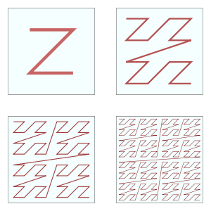
Because of their huge data volumes, LIDAR data are commonly distributed in “tiled” file formats. Datasets can be distributed in dozens to tens of thousands of sub-files, each with ad-hoc naming conventions. Meanwhile, inside of a powerful database like MapD, you probably want to get rid of arbitrary tiling schemes.
While utilities are available to combine GeoJSON files, the simplest current method is to generate CSV tabular files which are directly appendable. If file size is a concern, these can be gzipped, and MapD can read directly from the compressed file.
In addition to straight conversion, the script below illustrates the calculation of some useful attributes with PDAL.
- The first is the ‘smrf’ - for “Simple Morphological Filter” and affectionately known as ‘smurf.’ This applies a specific algorithm to calculate terrain ground surfaces, tagging the identified points with Classification=2.
- The “hag” filter computes a ‘height above ground’ for each point. This comes as a new attribute with the name HeightAboveGround.
- The third filter applies Morton ordering to the point stream, also known as Z-ordering. This has the nice property of allowing quick LIMIT queries in SQL to return a point set which contains spatially well-distributed samples.
import glob, os
# specify path to laz files and wildcard
filespec = “laz/*.laz"
# create PDAL format specification for outputs
fieldspec = 'X:7,Y:7,' # keep all 7 decimal places
fieldspec += 'Z:2,' # keep 2 places of precision
#integers or integer codes
fieldspec += ‘Intensity:0,ReturnNumber:0,’
fieldspec += ‘NumberOfReturns:0,Classification:0,'
# a newly-computed attribute, with 2 decimal places
fieldspec += 'HeightAboveGround:2'
for counter, file in enumerate(glob.glob(filespec)):
outfile = file.replace('.laz','.csv')
print('Working on file {}: {}'.format(counter, file))
# assuming local install, for docker, please see above
!pdal translate -i {file} -o {outfile} \
-f filters.smrf -f filters.hag \
-f filters.mortonorder \
--writers.text.keep_unspecified="false" \
—writers.text.order={fieldspec}
Importing Geodata to MapD
Once you have your geodata in a format and coordinate system supported by MapD, you have several import options.
Geo Formats With Server Access. As of 4.0 MapD’s “COPY FROM” has some new geo options. The syntax is simple:
COPY lidar_geo from ‘/demo/tahoe/merged_lidar_points.geojson' WITH (geo = ‘true’);
Note the new WITH (geo = ‘true') is required for import from geoJSON or shapefiles, which is a one-step process. Also, a quoted full path from root is typically required (assuming you aren’t running from the mapd bin directory).
Tabular-to-Geo. If you have elected to use CSV files, a two-step process is required. You’ll first need to create an empty table with the appropriate schema, then import *without* the geo option.
What’s pretty slick is that if you create a table with a point feature type, MapD can merge adjacent x & y columns containing the geocoordinates. Just be sure to specify your coordinate system’s SRID in the table creation ( GEOMETRY(POINT, 4326) ), or you will by default get an undefined coordinate system which will not correctly interoperate with defined ones.
CREATE TABLE jekyll_lidar (pid BIGINT, p GEOMETRY(POINT, 4326), z FLOAT, Intensity FLOAT, ReturnNumber INTEGER, NumberOfReturns INTEGER, Classification SMALLINT);
COPY jekyll_lidar FROM ‘/home/mapdadmin/demo/jekyll/2016_PostMatthew_GA_mastercat.csv';
Python Client. If you don’t have command line server access, you can use the pymapd library to run “copy from” within Python. Assuming you have a database connection global variable (see sample notebooks), the required routine would look like this:
import PyMapD, sys
def loadLIDAR(table_name, source_file):
global connection
query = 'COPY %s from \'%s\' WITH (geo = \'true\');' \
% (table_name, source_file)
try:
connection.execute(query)
except:
print ("Error creating table:", sys.exc_info()[0])
raise
loadLIDAR('lidar_geo', '/demo/tahoe/merged_lidar_points.shp')
The only tricky part is the need to \ escape the required single quotation marks in constructing the query string.
Visualizing LIDAR in MapD Immerse
Finally, the fun part! Once your data are in MapD, you have many visualization options. We’ll look at this in more detail in future posts exploring and analyzing the data. But to start, try creating a “Geo Heatmap.” This defaults to hexagons which you can rescale at will interactively. I’ve found this gives a smoother surface depiction than directly mapping the raw points.
- Launch Immerse and add a Geo Heatmap Chart
- Set your data source to your LIDAR points table
- Set your “dimensions” of latitude and longitude to your point field name (p in example above)
- Set your color to “Z” maximum elevation
Voila! - you should get a surface representation of the tops of objects in your area of interest.
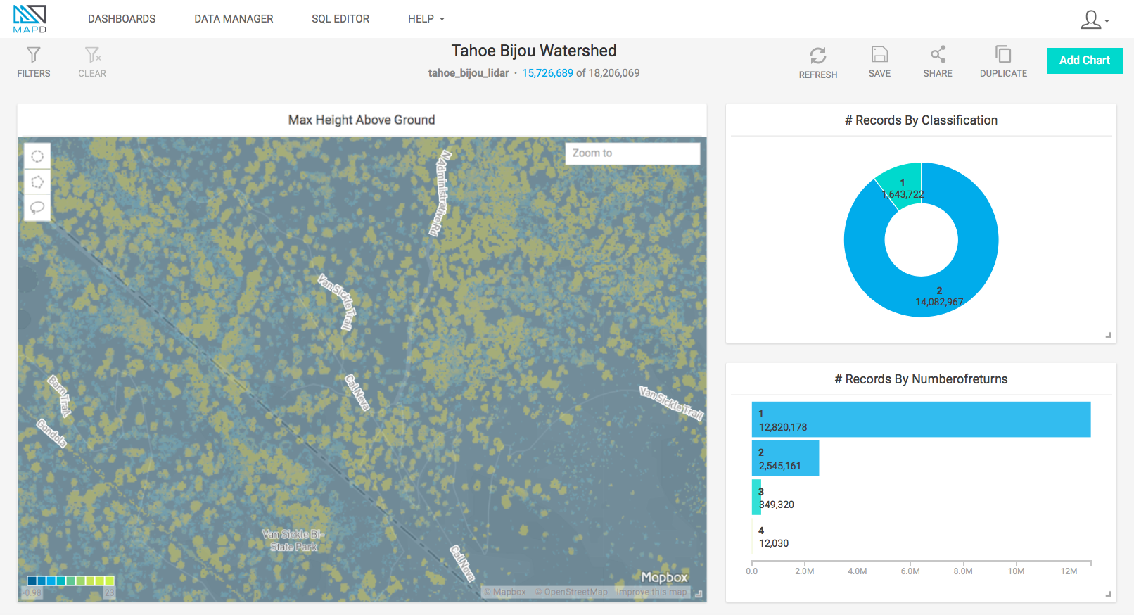
Then adjust your “Bin Pixel Size” to be as small as possible without showing gaps between the points. You may need to adjust this a bit depending on the map scales you wish to represent.
You may want to try experimenting with different basemaps. Using satellite imagery as a base can help you understand which objects your points represent. But this tends to make the points themselves a bit difficult to see. For this reason, you may just stick to the default Light background map, switching manually to satellite at detailed scales.
Conclusions
Handling large datasets distributed as multiple files requires a bit of prep work. But your reward is that once in MapD, you can treat such datasets as a single simple table - blazingly fast.
In my next installment, I’ll cover cross-filtering and spatial analyses of LIDAR using “point in polygon” techniques.


