Scaling Pandas to the Billions with Ibis and MapD
Download HEAVY.AI Free, a full-featured version available for use at no cost.
GET FREE LICENSE
Last week, Quansight announced that they had merged their work on the MapD backend for Python Ibis, which we sponsored as part of Quansight’s Sustainable Open Source model. With MapD, Ibis allows for scaling the familiar pandas DataFrame API into the billions of records at interactive speed. Here’s a first look at what you can expect.
Ibis: dplyr’s younger brother
Many enterprises adopting R use tidyverse packages, which provide a set of standardized workflows for manipulating tabular data. The Ibis project is similar in scope, abstracting over how and where the data is stored and thus allowing users to continue to use familiar Python and pandas idioms.
By providing a common interface for disparate data systems, like relational databases and Hadoop, users can focus on the business problem at hand, rather than think about the differences between data storage platforms or small differences in SQL dialects.
Setup
Given that the MapD backend to Ibis was merged just days ago, I’ll be working against the master branch of the Ibis project on GitHub, but a new version of Ibis containing the MapD code should be available in the coming weeks. To follow along with this post:
- Install the Conda environment
- Use the ‘All in One’ script to build a Docker environment with MapD
The Docker environment builds MapD Community Edition for CPU, which allows everyone to understand how MapD and Ibis work together without requiring a GPU. If you do have access to MapD running in a GPU environment, Ibis will work there also (fantastically so!), which I will demonstrate later in the post.
Connecting to MapD and Accessing Data
Connecting to MapD using Ibis is similar to other Python database packages:
#Connect to Docker environment
#Make sure to note which database you want to connect to:
#data loaded to "ibis_testing" automatically
#but frequently can be "mapd" database
import ibis
conn = ibis.mapd.connect(host="localhost", port = "9091", \
user="mapd", password="HyperInteractive", database="ibis_testing")
The list_tables method provides a list of the tables in the selected database:
#List tables in database
conn.list_tables()
['diamonds', 'batting', 'awards_players', 'functional_alltypes']
To start working with a table, we use the conn.table() method to create a reference; this does not bring the table local, as Ibis is lazy-evaluated by default. The only time we will bring data local is when we explicitly ask for a local copy.
#Create reference to table `batting`
#Note that this is a reference, it does not bring the table local
batting = conn.table('batting')
batting.info()
Table rows: 101332
Column Type Non-null #
------ ---- ----------
playerID String(nullable=True) 101332
yearID int64 101332
stint int64 101332
teamID String(nullable=True) 101332
lgID String(nullable=True) 100595
G int64 101332
AB int64 101332
R int64 101332
H int64 101332
...
Selecting Columns, Filtering and Grouping
Now that we’ve defined table batting (source: batting table from the ever-popular Lahman baseball database), we can now start to work with it in Ibis in a similar manner to a pandas dataframe. To select a single column, we can use the familiar <df>.<column> syntax or specify multiple columns using array indexing. Grouping and filtering are accomplished by method chaining:
#select a single column using dot notation, multiple using pandas array indexing
#conn.execute explicity asks for a local copy
player = conn.execute(batting.playerID)
player_year_game = (batting[["playerID", "yearID", "G"]]
.group_by(["playerID", "yearID"])
.aggregate(batting.G.sum().name("games_played"))
)
conn.execute(player_year_game.head())
playerID yearID games_played
0 whitnar01 1884 23
1 hoffojo01 1885 3
2 davisbe01 2002 80
3 freemma02 1988 11
4 arntzor01 1943 32
If you’re comfortable with SQL or just curious about what’s going on under hood, you can print out the generated SQL using conn.compile():
print(conn.compile(player_year_game))
SELECT "playerID", "yearID", sum("G") AS games_played
FROM (
SELECT "playerID", "yearID", "G"
FROM batting
) t0
GROUP BY playerID, yearID
The code above represents just a tiny sliver of the functions that Ibis supports with the MapD backend. With the exception of window functions and user-defined functions (which MapD Core doesn’t currently support), if you can write it in SQL then it can probably be accomplished using Ibis. Everything from filtering (WHERE), INNER/OUTER joins, subqueries, conditional logic (CASE WHEN) is probably possible and very similar to how it’s done using pandas.
Scaling Into the Hundred-Millions to Billions of Records
While the batting dataset is an easy starting point to get familiar with the Ibis workflow, its 100,000 records barely strain a spreadsheet, let alone a pandas dataframe, even on the most modest of computers. To illustrate the true power of Ibis backed by MapD, we once again turn to the billion-row Taxi dataset.
With a few additional data appends we’ve made internally, the Taxi dataset is 1.3 billion rows by 64 columns, occupying 192 GB at rest with gzip compression. Suffice to say, no matter how much CPU RAM your machine has, trying to process this data using a regular pandas dataframe is going to be a bad time!
Suppose we wanted to calculate tipping percentage for some arbitrary group of rides:
In the taxilim statement, I limit to the five columns that I’m actually going to use; this is a good practice in general for MapD, as MapD is a columnar SQL engine and explicitly declaring your columns minimizes data loaded to the GPU. From that smaller table, I can add a filter for just the boroughnames that start with ‘B’, as well as rides where the temperature is greater than 80. Finally, I want to calculate the average tip by boroughname and the weather conditions using group_by() and aggregate().
Running the statement without an execute() statement shows the DAG of the Ibis expression:
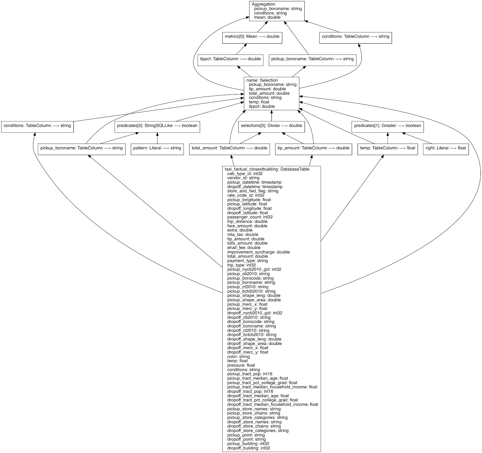
Looking at the generated SQL, Ibis writes the the statement like I might have written myself:
Finally, we can execute the expression and get our answer:
Writes Like Pandas, Scales To All The Hardware You Can Provide
How Ibis scales with MapD backend is a function of the hardware being used: the more GPUs you add, the more data you can process interactively within MapD. With 2 NVIDIA K80 GPUs, I was seeing sub-second response times for queries on 900MM records without the need for any table indexing, and 1.27 s ± 250 ms for the entire dataset.
But more importantly than just the raw speed, Ibis meshes the flexibility of working with pandas with the scalability of modern cloud and datacenter hardware to provide a very familiar workflow in data science. I’m tremendously impressed with Ibis as an open-source project and especially with the work that Quansight did to develop the MapD backend. I can’t wait to see how both MapD and Ibis evolve once the larger community gets involved!