Re-sampling Minute-Level Activity From Interval Data
Download HEAVY.AI Free, a full-featured version available for use at no cost.
GET FREE LICENSEPrior to joining OmniSci, I did a lot of big data reporting. One of the worst reports to calculate was taking data stored as intervals (e.g., start/end time for a car ride, session duration on a website, etc.) and re-sampling the data to minute-level usage. Due to the size of the dataset, the interval data was stored in a Hadoop cluster, and using Hive and/or Spark to generate the report was the obvious choice. Unfortunately, the trade-off for using those high-level APIs was awful performance, both on an I/O and clock-time basis.
An alternative I never considered until I started at OmniSci was using GPUs, along with a slightly different algorithm, to dramatically lower the time-to-report. This blog post will outline the Hive/Spark method I used, along with its performance traps, and a much-improved alternative using OmniSci Core (and a simpler algorithm) to resample interval data.
Method 1: Hive UDF along with EXPLODE
For the most part, Apache Hive is a godsend. Being able to use SQL on massive amounts of tabular data without the need to write MapReduce code brought big data analysis and reporting to tens of thousands of business users. But the flexibility of Hive can also have difficult I/O properties; eventually, you can’t just add more hardware and get better performance (whether your data center runs out of space or you run out of cloud budget).
One of the biggest offenders on this flexibility vs I/O performance trade-off in Hive is the EXPLODE function. The EXPLODE function is a table-generating function; in contrast to most functions in SQL, which take 0 or more inputs and return a record-level output, a table-generating function takes inputs from a single row but can return multiple rows. The use of table-generating functions most frequently occurs with complex data types such as arrays and maps, where multiple values can exist within a single (row, column) location and the user would like to “pivot” the results.
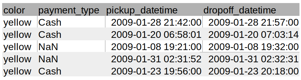
Take the following example, a small sample of rows and columns from the billion-row Taxi dataset:
Hive can work with collection types such as arrays, so re-sampling this data into minutes can be calculated using the following steps:
- Apply (user-defined) function to get an array of minutes during which the ride occurred
- Use EXPLODE function in Hive to “rotate the array” into rows in a column
- GROUP BY minute column, count number of rows
The algorithm described above is easy to write in Hive, but its I/O performance characteristics aren’t very pleasant. Let’s start by creating the array of minutes:
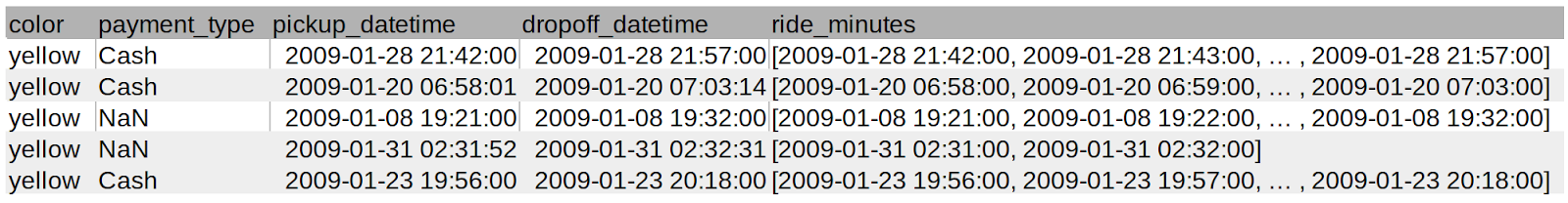
This operation isn’t too bad; projecting columns in a query is pretty much a given for all but the simplest queries. But once we EXPLODE the ride_minutes column, the I/O performance problem becomes evident:
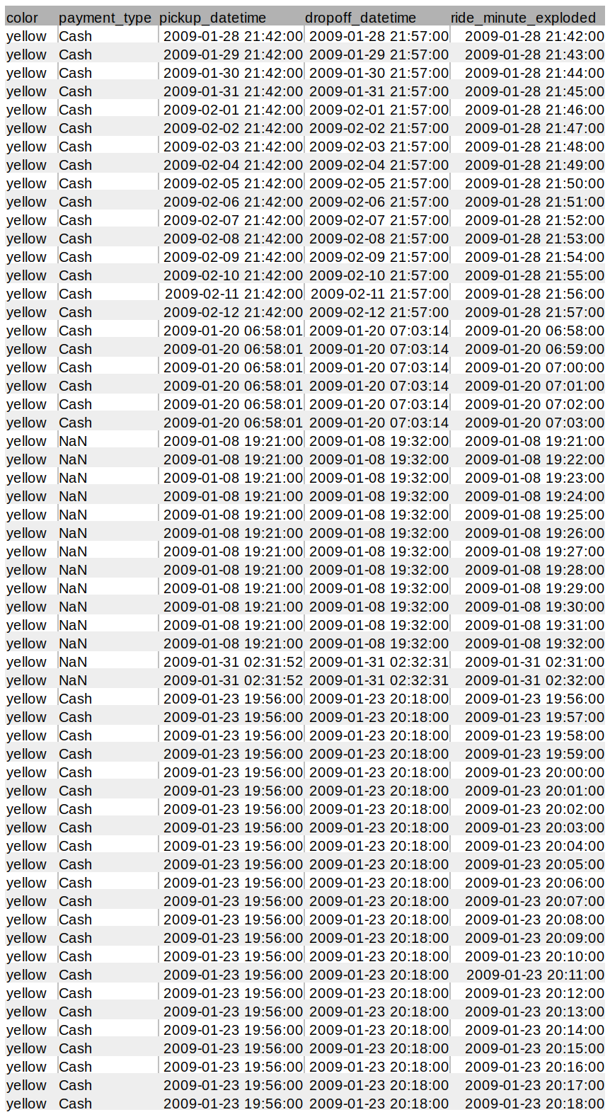
We went from a 5 row x 5 column sample dataset to 59 rows x 5 columns, a 12x increase in rows! If you’re lucky, an operation like this will only cause a write to disk (slow!), but the worst case scenario is that the JVM will crash if the results won’t fit inside the JVM memory. If you crash the JVM then you get to start the report over, trying different JVM memory settings and hoping the next run doesn’t crash.
Once you have this ‘exploded’ table, however, the GROUP BY statement will run pretty fast assuming you don’t have data skew. Unfortunately, you will almost certainly have data skew as human behavior skews to when people are awake (and meal times, rush hour, etc.). So 99% of your Hive workers will complete, and you’ll wait for what seems like forever for the last handful of workers to process the majority of the data and return the report.
Method 2: Calculate Rides Per Minute Directly
With the example above, I’ve shown that a straightforward way to write the Hive query has very poor I/O performance characteristics. An alternative to do this calculation would be the following:
select
color,
payment_type,
count(*) as rides
from nyctaxi
where '2010-01-03 17:00:00' between pickup_datetime and dropoff_datetime
group by 1,2
This query doesn’t require creating 11x the number of rows; in fact, it doesn’t require creating any intermediate data at all. What a query like this does require is running many queries, one for each minute. So instead of a single query to process all of your data like in the Hive example, you might have 1,440 queries per day of data. It will then be up to the analyst to write a script to loop over the desired minutes and accumulate the results into a useful report.
If There’s a Better Algorithm, Why Not Use It In Hive?
So if the second method is better (where “better” is defined as less I/O intensive), why not just use that? As it turns out, this method is on the whole slower than the EXPLODE method, due to the batch nature of Hive. Every query draws from a pool of resources (managed by the YARN resource manager), and releases those resources when the query completes. By running 1000s of small queries instead of one large query, the amount of time spinning-up JVMs, releasing them, then spinning them up again can be considerable.
Adding to the JVM spin-up times is also query start-up time in general. Most Hadoop clusters are multi-tenant, meaning lots of different users are competing for resources. Jobs are put into a queue and processed first-in-first-out (by default); many a day was wasted as I waited for a gigantic query by someone else to finish processing so that my jobs would run.
Method 3: OmniSci Core on GPUs with Per-Minute Queries
A third alternative is to leave the Hadoop altogether. Using OmniSci Core on GPUs, we gain the following favorable properties:
- High-bandwidth GPU RAM for fast data throughput
- High core density of GPUs for calculation
- Compiled queries using LLVM
- Low average query start latency
With the four points above, we remove all of the issues with Hadoop around JVM startup/shutdown and query latency while being able to still use the “Minute query” approach, which minimizes I/O. Let’s take a look at how to solve this problem quickly using pymapd:
From a cold start of OmniSci Core, the 1,440 queries necessary for a one-day report takes 4 minutes 16 seconds; this includes the time to read the data to GPU RAM and compile the query using LLVM. Upon repeated tests, the process takes about 3.5 minutes, meaning a query for each report minute is being processed in roughly 140 ms on consumer-grade hardware (two NVIDIA 1080ti cards). This is all done without any column indexing or other performance optimizations.
Comparing the 3.5 minute report time using OmniSci Core to Spark, we see a roughly 30x increase in time under the most optimal conditions:
Even with caching the pyspark dataframe into CPU RAM and extensive tuning of the Spark cluster from the AWS defaults, each minute query still takes on average 4.23s across the 1,440 query workflow. While 4 seconds vs. 142 milliseconds isn’t that large for a single query, for a report like this of 1,440 queries, the difference of what can be accomplished in an 8-hour workday starts to become evident.
Is this really a fair benchmark?
Of course, once you mention a 30x performance improvement over another tool, inevitably the “This isn’t a fair comparison!” argument happens. For this stylized example, it’s absolutely a fair point. OmniSci is absolutely a specialized, high-performance database that does fewer operations than the more general-purpose Apache Spark. Two GPUs running on the same desktop/node (OmniSci) is a different computing paradigm than a 30-node distributed cluster (Spark on AWS). And rarely is any analytics platform single-tenant (both platforms in this example).
The absolute performance difference between OmniSci and Spark isn’t the important takeaway here. Rather, what is important to understand is that GPUs fundamentally change how you can approach analytics problems through their massive bandwidth and core density. If you have a problem that takes too long to run, uses more hardware than is reasonable, or you just can’t solve the problem at all with the tools available to you, think about whether you can use a GPU (with OmniSci, of course). You might just be surprised.